Microsoft Excel: Converting a summary table / crosstab back into data rows
Posted: - Modified: | geekI recently wanted to transform a summary table of the form:
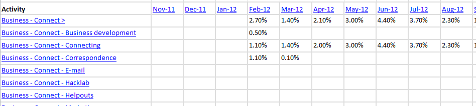
into a table with rows of (activity, date, value) so that I could add columns for year and month and then analyze the data using a pivot table.
It turns out that you can do this with another pivot table, yay! I followed this tutorial to convert my summary columns into data rows using Microsoft Excel 2010.
- Press Alt-D, P to get to the secret pivot table wizard that's different from the one you get from Insert > Pivot table.
- Choose Multiple consolidation ranges. Click Next.
- Choose I will create the page fields. Click Next.
- Select the range and add it. Go through the rest of the wizard to create a pivot table.
- Remove the row and column fields.
- Double-click on the total.
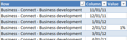
You should now see a table with the data from your crosstab.
Neato! Pivot tables are even cooler than I thought.
17 comments
Douglas G Pratt
2014-10-21T00:12:42ZThis is fantastic!
Dannylions
2014-10-21T16:27:52ZI don't understand a word... however - you are brilliant indeed my friend! Not only are you beautiful on the inside - you are on the outside and your brain is an intricate web of awesomeness!!!!!
Rajesh
2015-05-28T22:08:00ZYou're genius and this method is fantastic.
sachac
2015-05-29T03:59:03ZCredit belongs to the original tutorial writer! :) This is still, like, black magic for me.
darnfinanceguy
2015-06-29T23:36:14ZOMG. Saved me hundreds of hours of converting from essbase crosstab to database. Thanks!
excel learner
2015-12-16T04:18:04ZAmazing! This is awesome!!!!
RVM3
2016-05-15T13:45:06Znice
Dawn Carter-Little
2016-08-12T15:56:34ZGirl, You Rock! Like the Flintsones!!!!
So Helpful, save me tons of time
Adam
2017-01-21T18:33:11ZThis is an incredibly fantastic tip, thank you for taking the time to post it, like other, you saved me hours of work!
Ashley Nicholas (AshSandwich)
2017-05-08T12:25:41ZIncredible. The manual effort I've been putting into this task over the past 2 years was crazy. I don't know if I'm happy to have a solution, or mad that I didn't research it before! Thank you very much.
Sean O'Connell
2017-05-21T12:57:47ZThank you. Nice trick - very useful. In the past I have written VBA to denormalise such data.
Ashusen Tamang
2017-07-26T11:49:34ZThank you . This is awesome and fruitful tricks in Excel. It saves tremendous times in excel .
Keith Yap
2017-11-01T05:26:15ZThanks Sasha, great summary that helped me solve a problem quickly. I've written a bit more about how your method helped (complete with animated gif!)
https://medium.com/keith-ya...
Li Qian
2018-08-16T23:03:08ZNice Trick, you don't even need to remove the row and columns, just double click the grand total to drill down to the details.
Mark Eckman
2019-06-14T15:41:17ZOMG...You are awesome! That just saved me so much time. Thanks
v/r Mark Eckman
Senior Analyst Navy Medicine
Budi Setiawan
2020-01-28T17:04:25ZThanks a lot... Very usefull..
James
2024-04-04T05:56:02ZJust came back to this again. Absolute saviour!